Power Laws in Data and Optimization
From covariance spectra to scaling laws and spectral optimization
These notes follow one mathematical structure—a slowly decaying covariance spectrum—from its appearance in data to its consequences for learning curves, compute allocation, momentum, and matrix-valued optimization.
The goal is not only to derive a collection of scaling laws. It is to develop a reusable way of moving between empirical spectra, solvable high-dimensional models, random-matrix calculations, and experiments.
The organizing idea. Power-law covariance is visible in data, can persist through neural representation maps, and helps predict which optimization controls matter.
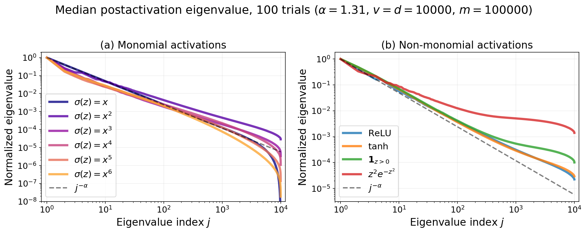
A recurring question throughout the course: which features of a power-law spectrum survive a nonlinear map, a learning dynamic, or an optimizer?
What to expect
The four modules build a single progression from data structure to optimizer design.
Power-Law Covariance
Learn to read empirical eigenspectra, formulate a power-law covariance model, and ask when nonlinear feature maps preserve its tail.
Compute-Optimal Scaling Laws
Turn a covariance spectrum into learning curves, separate approximation and optimization effects, and derive fixed-compute frontiers.
Momentum Schedules
Understand when constant momentum changes only a prefactor, when a schedule can change an exponent, and how those claims should be tested experimentally.
Muon and Spectral Optimizers
Start from the outer-product structure of a backpropagated weight gradient and analyze SignSVD and Muon through drift, volatility, and random-matrix deterministic equivalents.
Key skills
By the end, you should be able to:
Read a spectrum
Use log–log eigenspectra and effective slopes to distinguish a genuine power-law regime from finite-size cutoffs and other spectral structure.
Build a tractable model
Translate an empirical covariance hypothesis into a random-features or quadratic model that retains the modes relevant to learning.
Use the random-matrix toolkit
Work with resolvents and Stieltjes transforms, apply Gaussian integration by parts with directional derivatives, and interpret deterministic equivalents.
Analyze learning dynamics
Decompose error into descent and variance terms, derive Volterra-type equations, and identify the modes that dominate at a given time or compute budget.
Fit and audit scaling laws
Choose a compute convention, compare baselines, inspect structured residuals, and avoid mistaking a finite experimental window for an asymptotic law.
Reason about matrix-valued optimizers
Connect activation and backpropagation covariance to outer-product gradients, then study how orthogonalization or spectral preconditioning changes an update.
A visual through-line
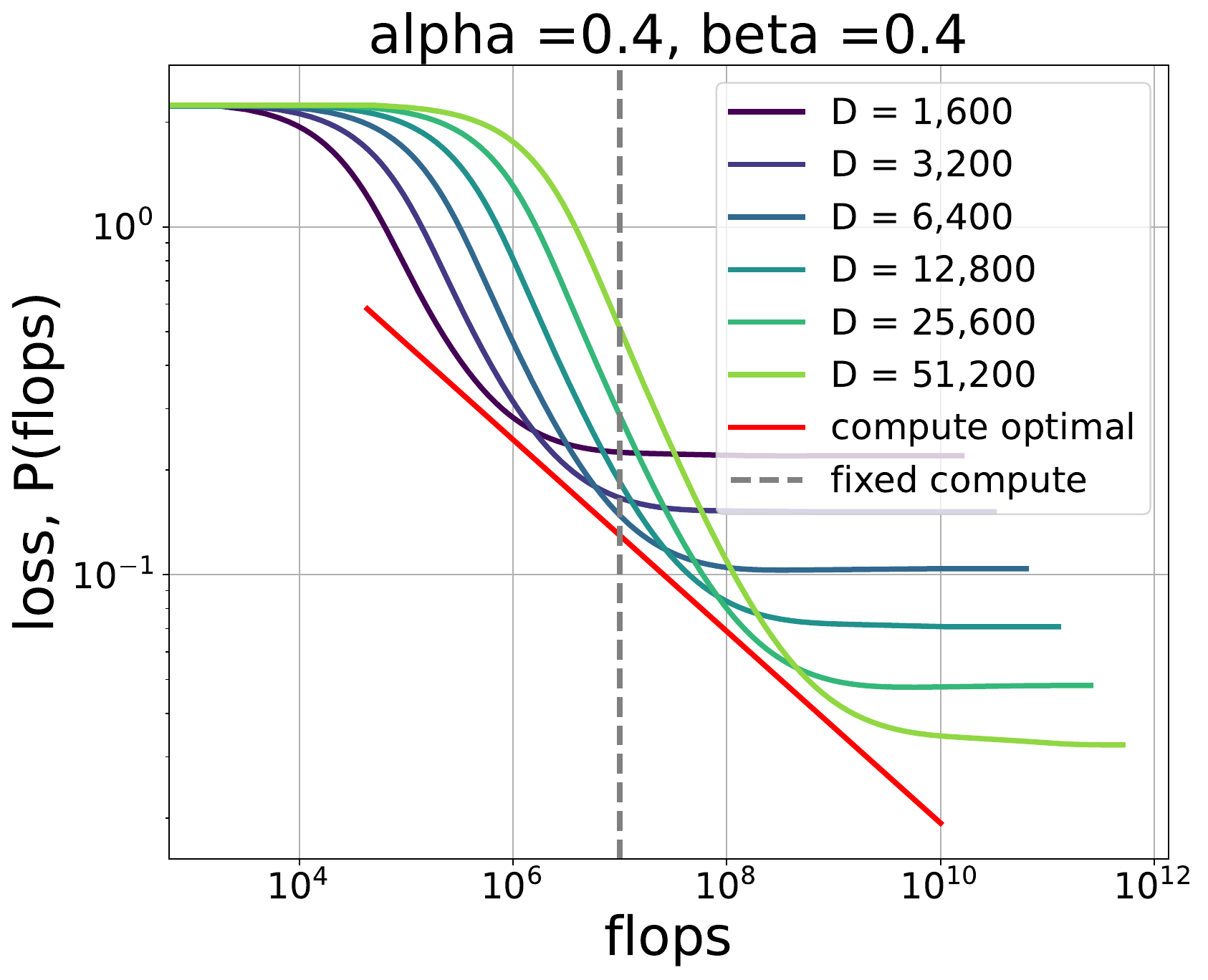
From spectra to compute. A covariance model produces learning curves at different model sizes; optimizing over size produces a compute frontier.
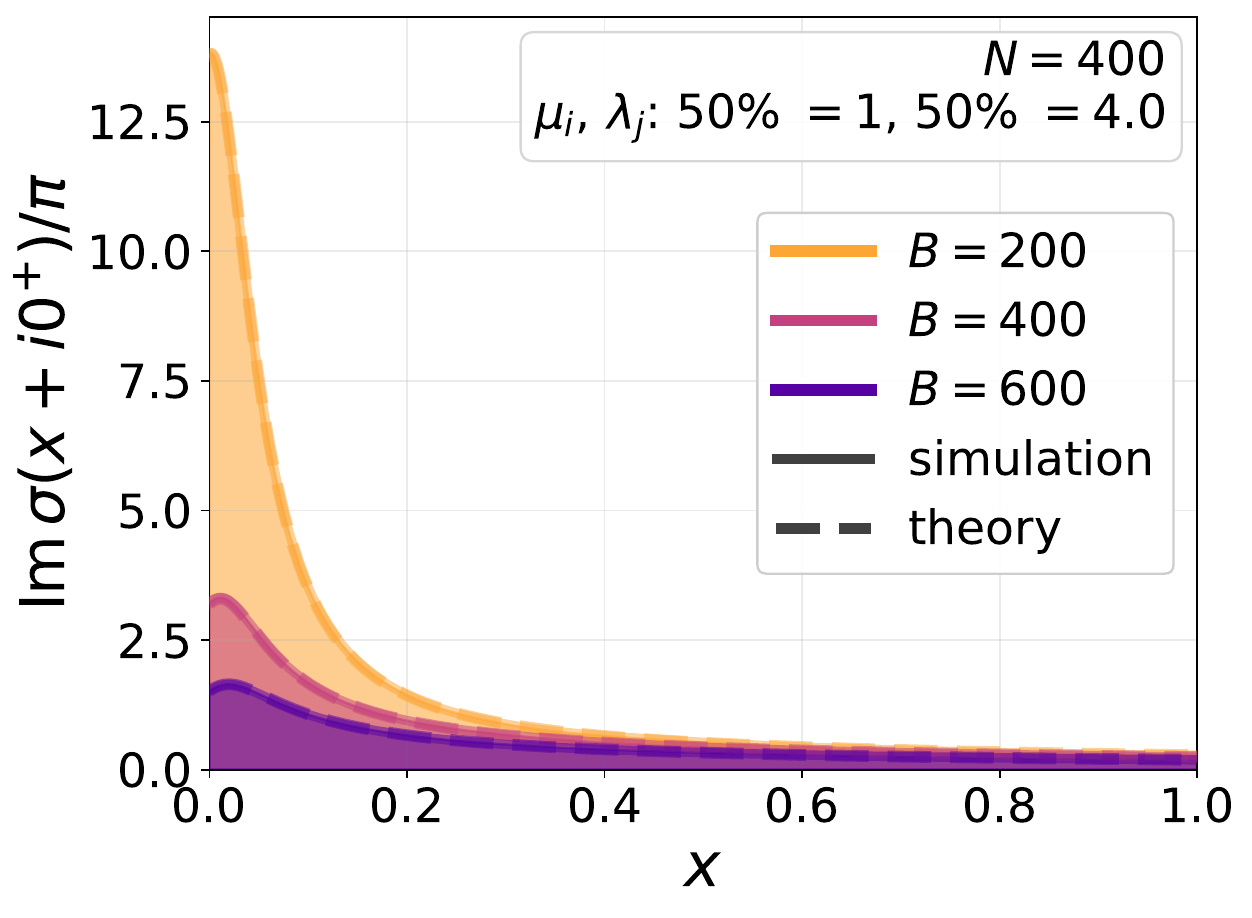
From matrices to predictions. Resolvent calculations convert a matrix-valued mini-batch update into spectral predictions that can be checked against simulation.
The modules are designed to be read in order, but each chapter also serves as a self-contained web note once the basic covariance picture is familiar.