Muon and Spectral Optimizers
When matrix geometry changes the effective covariance
Covariance now acts on a matrix gradient
The first three lectures treated power-law covariance as a structure on directions. For a weight matrix, the minibatch gradient \(G\) is itself a matrix. If
\[ \begin{gathered} G=U\operatorname{diag}(\sigma_1,\ldots,\sigma_r)V^\top,\\ \boxed{\operatorname{SignSVD}(G)=UV^\top.} \end{gathered} \]
SignSVD keeps the singular vectors and replaces every nonzero singular value by one. Muon approximates this operation with a few matrix multiplications.
How do covariance and batch size control gradient orthogonalization?
Backpropagation produces an outer product
Let
\[ \mathcal L(\theta) =\mathbb E_{(X,Y)} \left[\ell\!\left(F_\theta(X),Y\right)\right]. \]
For one layer, write \(z=Wa\) and \(\delta=\nabla_z\ell(F_\theta(X),Y)\). A perturbation \(dW\) gives
\[ \begin{aligned} d\ell &=\sum_{i,j}\delta_i a_j\,dW_{ij} =\langle\delta\otimes a,dW\rangle_F,\\ &\hspace{2.6em}\Longrightarrow\quad \boxed{\nabla_W\ell=\delta\otimes a.} \end{aligned} \]
A batch gradient has rank at most the batch size
For a minibatch of \(B\) examples,
\[ \boxed{ G_B=\frac1B\sum_{b=1}^B\delta_b\otimes a_b, \qquad \operatorname{rank}(G_B)\le B. } \]
Right geometry
The activation covariance acts on the input side of \(W\).
Left geometry
The backpropagated-error covariance acts on the output side.
Batch size limits the number of matrix directions visible to a spectral update.
A bilinear regression model preserves the matrix geometry
Take independent
\[ x\sim\mathcal N(0,\Sigma_{\rm in}), \qquad y\sim\mathcal N(0,\Sigma_{\rm out}), \]
and let \(\Delta=W-W_\star\). The single-sample loss is
\[ \ell(W;x,y) =\frac12\langle y\otimes x,\Delta\rangle_F^2. \]
Its gradient and population Hessian are
\[ \boxed{ \begin{aligned} \nabla_W\ell &=(y\otimes x)\langle y\otimes x,\Delta\rangle_F,\\ \mathcal K(H) &=\Sigma_{\rm out}H\Sigma_{\rm in}. \end{aligned} } \]
This is ordinary least squares whose matrix layout remains visible.
Two covariances create \(N^2\) paired modes
In the two covariance eigenbases,
\[ \begin{aligned} \Sigma_{\rm out}u_i&=\mu_i u_i, &\Sigma_{\rm in}v_j&=\lambda_jv_j,\\ \mathcal K(u_i\otimes v_j) &=\mu_i\lambda_j(u_i\otimes v_j),\\ \Delta&=\sum_{i,j}a_{ij}(u_i\otimes v_j). \end{aligned} \]
Consequently,
\[ \boxed{ \mathcal R(W) =\frac12\sum_{i,j}\mu_i\lambda_j a_{ij}^2. } \]
The eigenbasis is indexed by pairs \((i,j)\), so an \(N\times N\) matrix naturally has \(N^2\) spectral order parameters.
A spectral optimizer reshapes singular values
| update | matrix operation | action on \(\sigma\) |
|---|---|---|
| SGD | \(U\Sigma V^\top\) | \(\sigma\mapsto\sigma\); preserves the gradient hierarchy |
| power \(p\) | \(U\Sigma^pV^\top\) | \(\sigma\mapsto\sigma^p\); interpolates or reverses the hierarchy |
| SignSVD | \(UV^\top\) | \(\sigma\mapsto1\) on the nonzero subspace |
| instant Shampoo | \((GG^\top)^{\dagger/4}G(G^\top G)^{\dagger/4}\) | also \(\sigma\mapsto1\) |
| finite-NS Muon | \(\operatorname{NS}_K(G)\) | rapidly moves \(\sigma\) toward one |
Full flattening is one point on a broader spectral-power design axis.
SignSVD is the polar factor
For \(G=U\Sigma V^\top\),
\[ \boxed{ \operatorname{polar}(G) =(GG^\top)^{\dagger/2}G =UV^\top. } \]
It is basis-covariant:
\[ \operatorname{polar}(QGR^\top) =Q\,\operatorname{polar}(G)\,R^\top. \]
Entrywise SignSGD instead uses
\[ [\operatorname{sign}(G)]_{ij}=\operatorname{sign}(G_{ij}), \]
so it depends on the coordinate basis.
Muon separates a temporal choice from a spectral choice
A stylized Muon update is
\[ \begin{aligned} M_{t+1}&=\beta_{\rm mom}M_t+G_t,\\ W_{t+1}&=W_t-\eta\,\operatorname{NS}_K(M_{t+1}). \end{aligned} \]
It adds two operations to exact SignSVD:
- average gradients through momentum;
- approximate the polar factor without computing an SVD.
Instantaneous Shampoo gives the same polar factor because
\[ (GG^\top)^{\dagger/4}G(G^\top G)^{\dagger/4}=UV^\top. \]
Historical context: Carlson–Cevher–Carin (2015); Tuddenham–Prügel-Bennett–Hare (2022); Gupta–Koren–Singer (2018).
Newton–Schulz maps singular values toward one
Start with the cheap Frobenius normalization
\[ X_0=\frac{G}{\|G\|_F+\varepsilon}, \qquad \|X_0\|_{\rm op}\le1. \]
The classical polar iteration is
\[ X_{k+1} =\frac12(3X_k-X_kX_k^\top X_k), \qquad s_{k+1}=\frac12(3s_k-s_k^3). \]
Muon commonly uses five steps of
\[ X_{k+1}=aX_k+(bA_k+cA_k^2)X_k, \qquad A_k=X_kX_k^\top, \qquad (a,b,c)\approx(3.44,-4.78,2.03). \]
The large slope accelerates sharply near zero.
The clean model isolates the spectral operation
From now on:
\[ \boxed{ \beta_{\rm mom}=0, \qquad \operatorname{NS}_K(G)\longrightarrow\operatorname{polar}(G). } \]
The resulting algorithm is exact SignSVD.
This removes two separate approximation questions:
- no temporal averaging of successive gradients;
- no finite polynomial error in the polar map.
Momentum returns only after the covariance and batch-size effects are understood.
Dynamics
A matrix update still splits into descent and volatility.
One step is descent plus volatility
For residuals \(d_b=\langle y_b\otimes x_b,\Delta\rangle_F\), define
\[ \begin{gathered} G(\Delta)=\frac1B\sum_{b=1}^Bd_b(y_b\otimes x_b), \qquad S=\operatorname{polar}(G),\\ a_{ij}=u_i^\top\Delta v_j,\qquad s_{ij}=u_i^\top S v_j,\qquad q_{ij}=a_{ij}^2. \end{gathered} \]
Then exactly
\[ \boxed{ q_{ij}^+=q_{ij}-2\eta a_{ij}s_{ij}+\eta^2s_{ij}^2. } \]
Random matrix theory closes the dynamics
Define deterministic kernels by
\[ \mathbb E[a_{ij}s_{ij}\mid\Delta] \simeq \frac{\mathfrak d_{ij}}{\sqrt{\mathcal R}}q_{ij}, \qquad \mathbb E[s_{ij}^2\mid\Delta] \simeq\mathfrak v_{ij}. \]
Then
\[ \boxed{ q_{ij}(t+1) =q_{ij}(t) -\frac{2\eta\mathfrak d_{ij}(t)} {\sqrt{\mathcal R(t)}}q_{ij}(t) +\eta^2\mathfrak v_{ij}(t), } \]
with
\[ \mathcal R(t)=\frac12\sum_{i,j}\mu_i\lambda_jq_{ij}(t). \]
The random-matrix problem is to compute \((\mathfrak d_{ij},\mathfrak v_{ij})\) from the two covariances and \(B\).
The gradient Gram matrix is double Wishart
First decouple residuals from the Gaussian data:
\[ G_0=\frac1B YDX^\top, \qquad H_0=G_0G_0^\top. \]
Rewrite
\[ H_0=\frac1B YCY^\top, \qquad C=\frac1B DX^\top XD. \]
Conditioned on \(X\), the outer matrix is an ordinary sample covariance matrix with population matrix \(C\).
One Marchenko–Pastur computation is nested inside another.
When \(D=I\) and the dimensions are square, the resulting spectrum is the order-two Fuss–Catalan law.
Matrix Stein’s lemma avoids entrywise bookkeeping
Condition on \(C\) and set
\[ \widehat H_0=\Lambda^{1/2}WW^\top\Lambda^{1/2}, \qquad \widehat R=(\widehat H_0-zI)^{-1}. \]
For an independent Gaussian direction \(\widetilde W\),
\[ \boxed{ \mathbb E[F(W)W^\top\mid C] = \mathbb E[ (\partial_{\widetilde W}F(W))\widetilde W^\top \mid C]. } \]
The two directional derivatives are
\[ \partial_{\widetilde W}\widehat H_0 =\Lambda^{1/2} (\widetilde W W^\top+W\widetilde W^\top) \Lambda^{1/2}, \qquad \partial_{\widetilde W}\widehat R =-\widehat R(\partial_{\widetilde W}\widehat H_0)\widehat R. \]
Coherent contractions create the deterministic trace
Apply matrix Stein to \(F(W)=\widehat R\Lambda^{1/2}W\).
The independent direction produces two contractions:
\[ \mathbb E_{\widetilde W}[\widetilde W A\widetilde W^\top] =\frac1p\operatorname{tr}(A)I \quad\text{(coherent)}, \]
while the crossed contraction is an explicit \(p^{-1}\) matrix correction. The master equation is
\[ \boxed{ \mathbb E[\widehat R\widehat H_0\mid C] = \mathbb E\!\left[ q_p(z)\widehat R\Lambda -\frac1p\widehat R\widehat H_0\widehat R\Lambda \mid C \right], } \]
where
\[ q_p(z)=1-\frac1p\operatorname{tr}(\widehat R\widehat H_0). \]
The outer fixed point is a deformed MP equation
The incoherent correction vanishes at leading order, giving
\[ \widehat R(z) \simeq (\gamma_{\rm out}q(z)C-zI)^{-1}. \]
Therefore
\[ \boxed{ q(z)= \left[ 1+\int \frac{t}{\gamma_{\rm out}q(z)t-z}\,d\nu_C(t) \right]^{-1}. } \]
The normalized resolvent trace is
\[ m_{H_0}(z) =\frac1{\gamma_{\rm out}} \int\frac{d\nu_C(t)} {\gamma_{\rm out}q(z)t-z} +\frac{\gamma_{\rm out}^{-1}-1}{z}. \]
The inner law \(\nu_C\) comes from the same calculation applied to \(C=DX^\top XD/B\).
Anisotropy introduces two weighted traces
Set
\[ \sigma=\frac1B\operatorname{tr}(R\Sigma_{\rm out}), \qquad \widetilde\sigma =\frac1B\operatorname{tr}(\widetilde R\Sigma_{\rm in}). \]
The fixed point is
\[ \boxed{ \begin{aligned} \sigma &=\frac1B\sum_i\frac{\mu_i}{\widetilde s_1\mu_i-z}, & \widetilde\sigma &=\frac1B\sum_j\frac{\lambda_j}{s_1\lambda_j-z},\\ s_1&=\widetilde s_1\frac{\sigma}{\widetilde\sigma}, & \widetilde s_1\sigma&=f(\xi),\\ \xi&=(-2z\sigma\widetilde\sigma)^{-1/2}. \end{aligned} } \]
Here \(f(\xi)=1-\sqrt\pi\,\xi e^{\xi^2}\operatorname{erfc}(\xi)\) records the limiting residual-weight distribution.
The fixed point predicts the batch spectrum
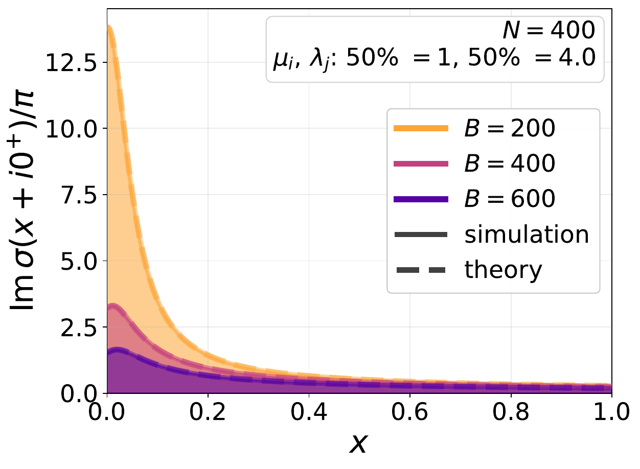
The fixed-point density matches Monte Carlo on both sides of the batch threshold.
The spectrum is not the descent
The normalized gradient has a residual diagonal
\[ \frac{G}{\sqrt{2\mathcal R}} =\frac1B Y\widehat D X^\top. \]
Replacing \(\widehat D\) by an independent diagonal with the same empirical law does not change the leading bulk spectrum.
But descent requires the overlap with the current error:
\[ \boxed{ \mathbb E[R(z)G\mid\Delta] \simeq c(z)\, R_{\rm eq}(z)\Sigma_{\rm out}\Delta\Sigma_{\rm in} \widetilde R_{\rm eq}(z). } \]
The dependence between residuals and data is precisely what makes this observable nonzero.
The same resolvent gives the descent coefficient
For a spectral transform \(\varphi\),
\[ \varphi(H)G =-\frac1{2\pi i}\oint\varphi(z)R(z)G\,dz. \]
Thus
\[ \boxed{ \mathfrak d_{ij} =-\frac{2\sqrt{\mathcal R}\,\mu_i\lambda_j}{\pi} \int_0^\infty x\,\varphi(2\mathcal R x)\, \operatorname{Im}\!\left[ \frac{\xi^2f(\xi)} {(\widetilde s_1\mu_i-z)(s_1\lambda_j-z)} \right]_{z=x+i0^+}\,dx. } \]
For SignSVD, \(\varphi(s)=s^{-1/2}\), so the current-risk dependence cancels.
Isotropy collapses every paired mode
Take
\[ \Sigma_{\rm in}=\Sigma_{\rm out}=I_N. \]
All \(N^2\) modes are exchangeable:
\[ \mathcal R(t+1) =\mathcal R(t) -2\eta\mathfrak d\sqrt{\mathcal R(t)} +\frac{\eta^2}{2}\mathfrak v. \]
| algorithm | drift \(\mathfrak d\) | volatility \(\mathfrak v\) |
|---|---|---|
| SignSVD | \(C(N/B)\) | \(\min\{B,N\}\) |
| SignSGD | \(\mathcal N_B/\sqrt\pi\) | \(N^2\) |
Here \(\mathcal N_B\sim\sqrt B\) and \(C(N/B)\) is a spectral moment of the fixed-point density.
SignSGD drift is controlled by density at zero
Separate one entry’s small signal from the diffuse residual:
\[ G_{pn} \approx \frac1B\sum_{b=1}^B \left[ y_{bp}^2x_{bn}^2\Delta_{pn} +y_{bp}x_{bn}\sqrt{2\mathcal R}\,z_b \right]. \]
A local limit theorem gives density convergence of the second term to \(Z\sim\mathcal N(0,s^2)\). For small \(\mu\), \(\mathbb E[\operatorname{sign}(Z+\mu)] =\sqrt{2/\pi}\,\mu/s+O((\mu/s)^3)\), so
\[ \boxed{ \mathfrak d_{pn}^{\rm SignSGD} =\frac{\mathcal N_B}{\sqrt\pi} \sim\sqrt{\frac B\pi}. } \]
SignSGD volatility is coordinatewise
Each entry of \(S=\operatorname{sign}(G)\) is \(\pm1\), so
\[ \boxed{ s_{pn}^2=1, \qquad \|S\|_F^2=N^2. } \]
\[ \eta_\star(t) =\frac{2\mathfrak d\sqrt{\mathcal R(t)}}{\mathfrak v}, \qquad \frac{\eta_\star^{\rm SignSVD}} {\eta_\star^{\rm SignSGD}} \asymp \begin{cases} \sqrt N,&B\ge N,\\ N/\sqrt B,&B\le N. \end{cases} \]
Their learning-rate scales differ even when tuned contractions agree.
Isotropy removes the reason to precondition
After tuning each method to its natural learning-rate scale,
\[ \text{SignSVD contraction} \asymp \text{SignSGD contraction} \]
up to absolute constants.
Muon’s spectral geometry becomes useful only when the covariance is anisotropic.
This sanity check prevents a normalization difference from being mistaken for an algorithmic advantage.
Half-anisotropy
Half-anisotropy turns \(N^2\) paired modes into \(N\) row norms.
One isotropic side removes one spectral index
Set
\[ \Sigma_{\rm in}=I_N, \qquad \Sigma_{\rm out} =U\operatorname{diag}(\mu_1,\ldots,\mu_N)U^\top. \]
Define the row-projected risks
\[ \boxed{ r_i(t)=\sum_{j=1}^Nq_{ij}(t) =\|\Delta_t^\top u_i\|^2, \qquad \mathcal R(t)=\frac12\sum_i\mu_i r_i(t). } \]
They satisfy
\[ r_i(t+1) =r_i(t) -\frac{2\eta\mathfrak d_i}{\sqrt{\mathcal R(t)}}r_i(t) +\eta^2\mathfrak v_i. \]
SignSVD volatility is a projection
Proposition. Let \(S=\operatorname{polar}(G)=U_rV_r^\top\). Then
\[ \boxed{ \|S^\top u_i\|^2 =u_i^\top P_{\operatorname{col}(G)}u_i. } \]
If \(B\ge N\) and \(G\) has full row rank, this equals one for every mode. If \(B<N\) and \(\operatorname{rank}(G)=B\), then
\[ 0\le\mathfrak v_i\le1, \qquad \sum_i\mathfrak v_i=B. \]
Orthogonalization cancels the singular values
Because \(S=U_rV_r^\top\),
\[ SS^\top =U_rV_r^\top V_rU_r^\top =U_rU_r^\top =P_{\operatorname{col}(G)}. \]
Therefore
\[ \|S^\top u_i\|^2 =u_i^\top SS^\top u_i. \]
For a general spectral map,
\[ SS^\top =U_r\operatorname{diag} \left(\varphi(\sigma_k^2)^2\sigma_k^2\right)U_r^\top, \]
so the volatility keeps a nontrivial spectral weight.
The map \(\sigma_k\mapsto1\) turns a difficult variance calculation into a projector identity.
Half-anisotropy leaves one population spectral sum
Set \(\gamma=N/B\). The reduced fixed point is
\[ \begin{aligned} \sigma &=\frac1B\sum_i\frac{\mu_i}{\widetilde s_1\mu_i-z}, & \widetilde s_1\sigma&=f(\xi),\\ \widetilde\sigma &=\frac{f(\xi)-\gamma}{z}, & s_1&=z+\frac{\gamma}{\widetilde\sigma}. \end{aligned} \]
\[ \boxed{ \begin{aligned} \rho_i(x) &=\frac1\pi\operatorname{Im} \frac1{\widetilde s_1(x+i0^+)\mu_i-x},\\ \mathfrak d_i &=\frac1\gamma\int_0^\infty\sqrt x\,\rho_i(x)\,dx,\\ \mathfrak v_i &=\int_0^\infty\rho_i(x)\,dx. \end{aligned} } \]
Large batches produce square-root drift
For \(B\ge N\),
\[ \boxed{ \mathfrak d_i=\sqrt{\frac{\mu_i}{\gamma}}, \qquad \mathfrak v_i=1. } \]
In algorithmic time,
\[ \frac{dr_i}{d\tau} =-2\sqrt{\frac{\mu_i}{\gamma}}\,r_i. \]
Thus
\[ \text{GD: }-\mathcal K(\Delta), \qquad \text{SignSVD: }-\mathcal K^{1/2}(\Delta). \]
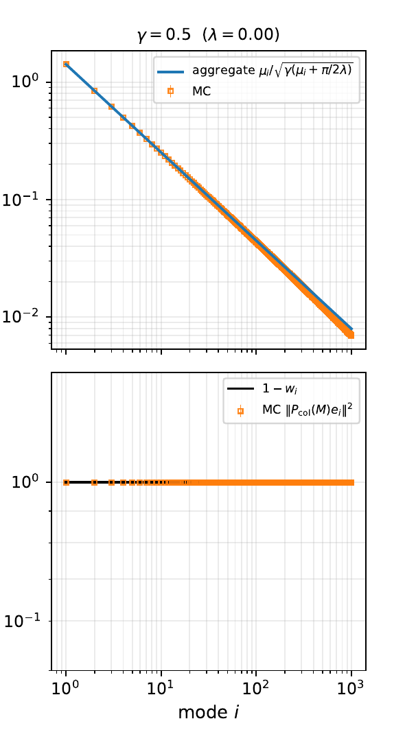
Small batches create a spectral resolution boundary
Define \(\Lambda\) by
\[ B=\sum_i\frac{\Lambda\mu_i}{1+\Lambda\mu_i}. \]
Then
\[ \mathfrak v_i =\frac{\Lambda\mu_i}{1+\Lambda\mu_i}, \]
and
\[ \mathfrak d_i\approx \begin{cases} \sqrt{\mu_i}\sqrt{B/N}, &\Lambda\mu_i\gg1,\\ \mu_i\sqrt{2\Lambda B/(\pi N)}, &\Lambda\mu_i\ll1. \end{cases} \]
The head is preconditioned; the unresolved tail returns to SGD-like drift.
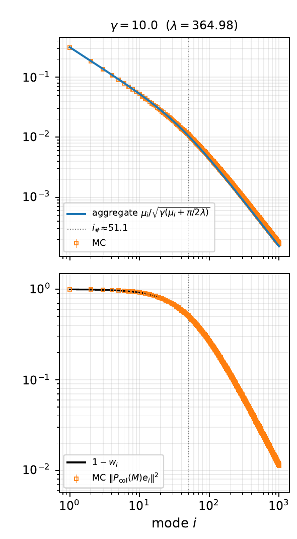
Power laws set the number of resolved modes
Take
\[ \mu_i=i^{-\alpha}, \qquad r_i(0)=i^{-\beta}, \qquad \alpha+\beta>1. \]
The boundary \(i_\#=\Lambda^{1/\alpha}\) obeys
\[ \boxed{ i_\#\asymp \begin{cases} B,&\alpha>1,\\ B/\log(N/B),&\alpha=1,\\ B^{1/\alpha}/N^{1/\alpha-1},&0<\alpha<1. \end{cases} } \]
For \(\alpha=\tfrac12\), \(i_\#\asymp B^2/N\): a batch of order \(\sqrt N\) resolves only order-one modes.
The batch selects between two spectral regimes
| mode range | SignSVD drift | SignSVD volatility |
|---|---|---|
| resolved head | \(\sqrt{\mu_i}\sqrt{B/N}\) | \(1\) |
| unresolved tail | \(\mu_i\sqrt{2\Lambda B/(\pi N)}\) | \(\Lambda\mu_i\) |
For comparison, half-anisotropic SignSGD retains
\[ \mathfrak d_i^{\rm SignSGD} =\frac{\mu_i\mathcal N_B} {\sqrt{\pi\overline\mu}}, \qquad \overline\mu=\frac1N\sum_i\mu_i. \]
Batch size is a spectral resolution scale, not only a variance-reduction parameter.
Compare algorithms at a common noise floor
For kernels \((\mathfrak d_i,\mathfrak v_i)\), define
\[ \mathcal S =\sum_i\frac{\mu_i\mathfrak v_i}{2\mathfrak d_i}, \qquad \boxed{\eta^\star=\frac{2\sqrt\epsilon}{\mathcal S}.} \]
Use this single constant learning rate throughout the run and measure
\[ t_{4\epsilon} =\inf\{t\ge0:\mathcal R(t)\le4\epsilon\}. \]
This avoids comparing two optimizers at the same numerical learning rate even though their update norms differ by powers of \(N\).
Square-root drift changes the time-to-accuracy exponent
Theorem (P.–Marshall–Benigni–Wang–Agarwala–P., 2026). Let \(\gamma=N/B\le1\), \(\mu_i=i^{-\alpha}\), \(r_i(0)=i^{-\beta}\), and \(\alpha+\beta>1\). Then
\[ t_{4\epsilon}^{\rm SignSVD} \asymp \begin{cases} \gamma N^{1-\alpha/2} \epsilon^{-\alpha/[2(\alpha+\beta-1)]},&\beta<1,\\ \mathcal S_{\rm SignSVD}\epsilon^{-1/2},&\beta>1, \end{cases} \]
while
\[ t_{4\epsilon}^{\rm SignSGD} \asymp \begin{cases} \dfrac{\pi N^2\overline\mu}{B} \epsilon^{-\alpha/(\alpha+\beta-1)},&\beta<\alpha+1,\\ \mathcal S_{\rm SignSGD}\epsilon^{-1/2},&\beta>\alpha+1. \end{cases} \]
The first SignSVD branch assumes \(0<\alpha<2\); boundaries carry logarithmic corrections.
Target structure decides whether orthogonalization helps
| target regime | range | comparison |
|---|---|---|
| tail-heavy | \(\beta<1\) | SignSVD is polynomially faster as \(\epsilon\to0\) |
| intermediate | \(1<\beta<\alpha+1\) | SignSGD may lead early; SignSVD wins at high accuracy |
| head-heavy | \(\beta>\alpha+1\) | both use the \(\epsilon^{-1/2}\) branch |
The mechanism is spectral:
\[ \mathfrak d_i^{\rm SignSVD}\propto\mu_i^{1/2}, \qquad \mathfrak d_i^{\rm SignSGD}\propto\mu_i. \]
Tail-heavy targets expose the different exponents
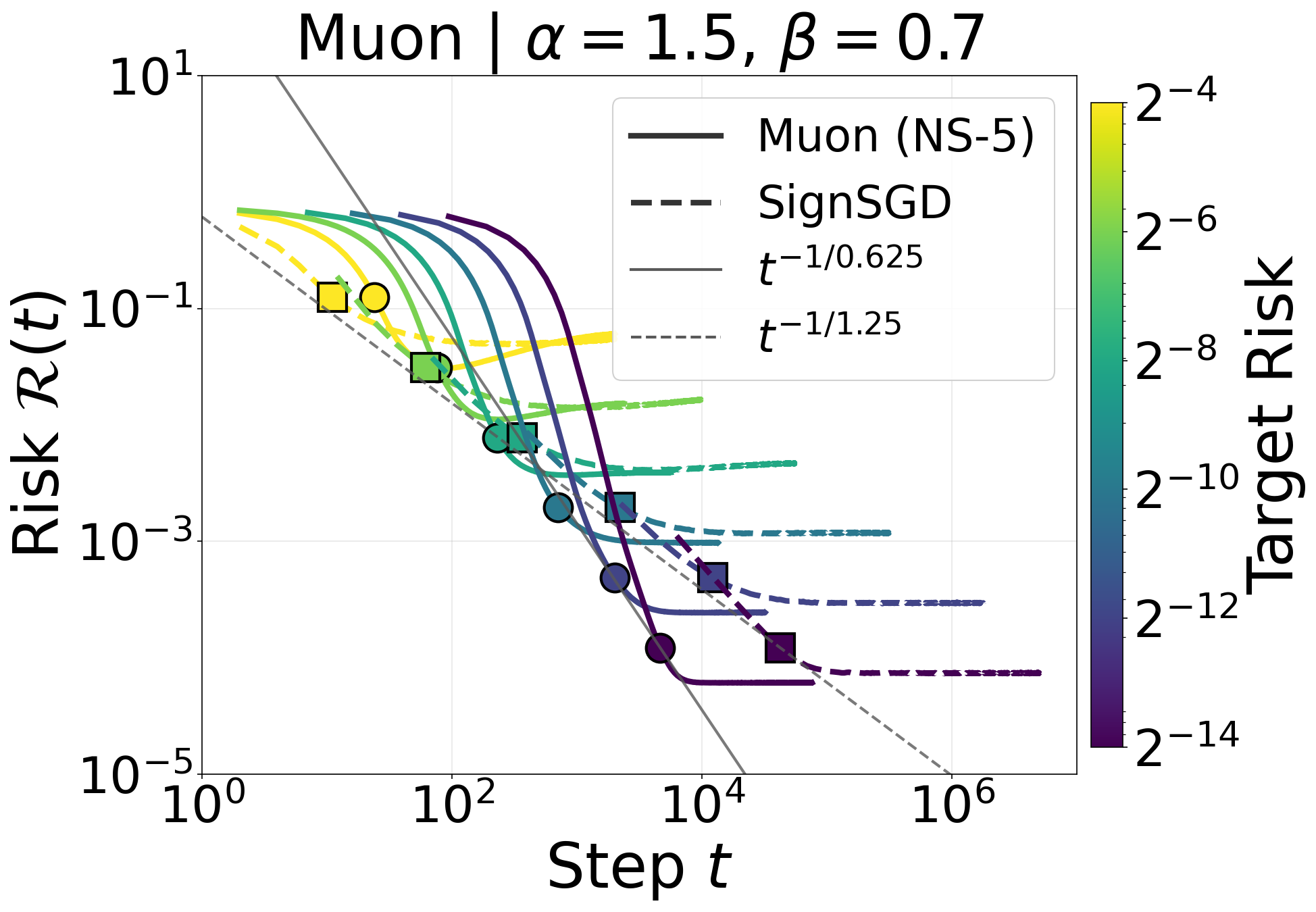
Tail-heavy example: \(\alpha=1.5\), \(\beta=0.7\), \(N=1024\), \(B=2048\). Solid: no-momentum Muon NS-5. Dashed: SignSGD.
Momentum
Momentum is a separate temporal question.
Five Newton–Schulz steps already track SignSVD
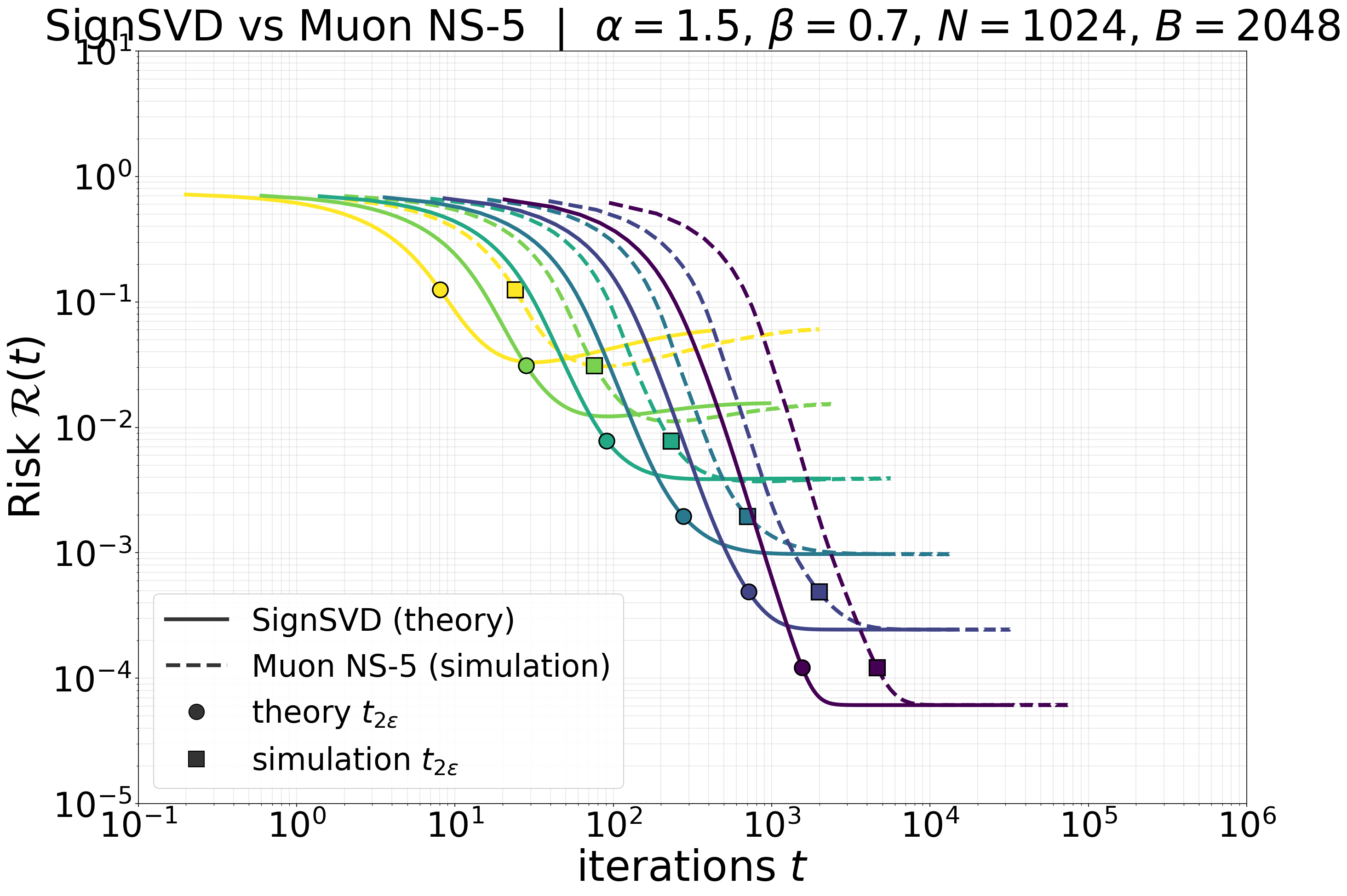
In this model, the finite polar approximation is a small correction to the exact SignSVD dynamics.
Momentum inflates integrated volatility
Suppose \(\operatorname{Corr}(\xi_t,\xi_{t+k}) \approx\beta_{\rm mom}^{\,k}\). Then
\[ \boxed{ \begin{aligned} \operatorname{Var}\!\left(\sum_{t=1}^T\xi_t\right) &\approx Tv\left(1+2\sum_{k\ge1}\beta_{\rm mom}^k\right)\\ &= Tv\,\frac{1+\beta_{\rm mom}}{1-\beta_{\rm mom}},\\ \text{SD inflation} &=\sqrt{\frac{1+\beta_{\rm mom}}{1-\beta_{\rm mom}}}. \end{aligned} } \]
At fixed learning rate, momentum raises the noise floor
Define \(\mathcal N_{\rm eff}\) by \(\mathcal R_\infty\approx(\eta\mathcal N_{\rm eff}/2)^2\).
| \(\beta_{\rm mom}\) | measured \(\mathcal N_{\rm eff}\) | AR(1) prediction |
|---|---|---|
| \(0\) | \(9.97\) | baseline |
| \(0.90\) | \(36.90\) | \(36.59\) |
| \(0.95\) | \(52.49\) | \(52.43\) |
| \(0.99\) | \(117.33\) | \(118.42\) |
Fixed learning rate. Each run fixes \(\eta\); reaching floor \(\epsilon\) requires \(\eta^\star=2\sqrt\epsilon/\mathcal N_{\rm eff}\) (model-specific).
Selected references
Elliot Paquette, Noah Marshall, Lucas Benigni, Guangyuan Wang, Atish Agarwala, and Courtney Paquette. “Phases of Muon: When Muon Eclipses SignSGD.” 2026. arXiv:2605.09552
Keller Jordan et al. “Muon: An Optimizer for Hidden Layers in Neural Networks.” 2024. Online article
Jingyuan Liu et al. “Muon Is Scalable for LLM Training.” 2025. arXiv:2502.16982
Vineet Gupta, Tomer Koren, and Yoram Singer. “Shampoo: Preconditioned Stochastic Tensor Optimization.” ICML 2018. PMLR
Ke Liang Xiao, Noah Marshall, Atish Agarwala, and Elliot Paquette. “Exact Risk Curves of SignSGD in High Dimensions.” ICLR 2025. OpenReview
Three mechanisms explain the spectral gain
Matrix structure
\[ G_B=\frac1B\sum_bd_b(y_b\otimes x_b) \]
The batch gradient is low rank and has two covariance geometries.
Preconditioning
\[ \mu_i\longmapsto\sqrt{\mu_i} \]
Resolved modes receive square-root covariance drift.
Resolution
\[ \sum_i\mathfrak v_i=B \]
The batch determines which modes are preconditioned.
Muon’s matrix operation matters when anisotropy and target mass make weak covariance directions the optimization bottleneck.